Model assessment and variable selection

Author

therimalaya

Published

March 5, 2017

Whenever we add a variable in our model, we are not only adding information but also noise that clutter the information and makes the analysis difficult. Simpler model is always better since they contain less noise and they are easy to interpret. In real life, things are not that simple. But relax, there are statistical methods that make model assessment and perform variable selection and gives optimal set of variables for us.

Here, I will discuss how to compare model to know which one is better than other. This model assessment help us to select a model with few variable that can perform as good as a model with large number of variables. Here comes the idea of variable selection. I will try to explain these concepts with an example. For the example I will use mtcars data set which is available in R by default. Following are two well know procedure of selecting subset of variables,

Best subset method

Best subset procedure selects best regression model by running all possible subset of variables. When number of variable is large, the possible combinations of candidate subset become huge. For example, for 2 variable case (\(X_1\) and \(X_2\)), there are 4 possible subsets – 1 with no predictors, 2 with single predictors and 1 with both predictors. Similarly, if there are 4 variable case (\(X_1, X_2, X_3\) and \(X_4\)), there will be 16 possible subset. In general, fitting all possible subset of large number of predictors becomes computationally intensive.

Once, all the possible model is fitted, they are compared based on some criteria. This model assessment may based on various criteria such as coefficient of determination (\(R^2\)), adjusted \(R^2\), Mallow’s CP, AIC and BIC. In R, leaps package can be used for performing this operation. Lets dig into our mtcars example.

Fitting a complete model:

full.model <- lm(mpg ~ ., data = mtcars)
smry <- summary(full.model)

smry


Call:
lm(formula = mpg ~ ., data = mtcars)

Residuals:
    Min      1Q  Median      3Q     Max 
-3.4506 -1.6044 -0.1196  1.2193  4.6271 

Coefficients:
            Estimate Std. Error t value Pr(>|t|)  
(Intercept) 12.30337   18.71788   0.657   0.5181  
cyl         -0.11144    1.04502  -0.107   0.9161  
disp         0.01334    0.01786   0.747   0.4635  
hp          -0.02148    0.02177  -0.987   0.3350  
drat         0.78711    1.63537   0.481   0.6353  
wt          -3.71530    1.89441  -1.961   0.0633 .
qsec         0.82104    0.73084   1.123   0.2739  
vs           0.31776    2.10451   0.151   0.8814  
am           2.52023    2.05665   1.225   0.2340  
gear         0.65541    1.49326   0.439   0.6652  
carb        -0.19942    0.82875  -0.241   0.8122  
---
Signif. codes:  0 '***' 0.001 '**' 0.01 '*' 0.05 '.' 0.1 ' ' 1

Residual standard error: 2.65 on 21 degrees of freedom
Multiple R-squared:  0.869, Adjusted R-squared:  0.8066 
F-statistic: 13.93 on 10 and 21 DF,  p-value: 3.793e-07

Here, we can see that the model has explained almost 86.9 percent of variation present in mpg, but non of the predictors are significant. This is a hint of having unnecessary variables that has increased model error. Using regsubsets function from leaps package, we can select a subset of predictors based on some criteria.

library(leaps)
best.subset <-
  regsubsets(
    x      = mtcars[, -1],     # predictor variables
    y      = mtcars[, 1],      # response variable (mpg)
    nbest  = 1,                # top 1 best model
    nvmax  = ncol(mtcars) - 1, # max. number of variable (all)
    method = "exhaustive"      # search all possible subset
  )
bs.smry <- summary(best.subset)

We can combine following summary output with a plot created from additional estimates to get some insight. These estimates are also found in the summary object. The output show which variables are included with a star(*).

pander::pander(bs.smry$outmat)
bs.est <- data.frame(
  nvar   = 1:(best.subset$nvmax - 1),
  adj.r2 = round(bs.smry$adjr2, 3),
  cp     = round(bs.smry$cp, 3),
  bic    = round(bs.smry$bic, 3)
)
bs.est <- tidyr::gather(bs.est, "estimates", "value", -nvar)

	cyl	disp	hp	drat	wt	qsec	vs	am	gear	carb
1 ( 1 )					*
2 ( 1 )	*				*
3 ( 1 )					*	*		*
4 ( 1 )			*		*	*		*
5 ( 1 )		*	*		*	*		*
6 ( 1 )		*	*	*	*	*		*
7 ( 1 )		*	*	*	*	*		*	*
8 ( 1 )		*	*	*	*	*		*	*	*
9 ( 1 )		*	*	*	*	*	*	*	*	*
10 ( 1 )	*	*	*	*	*	*	*	*	*	*

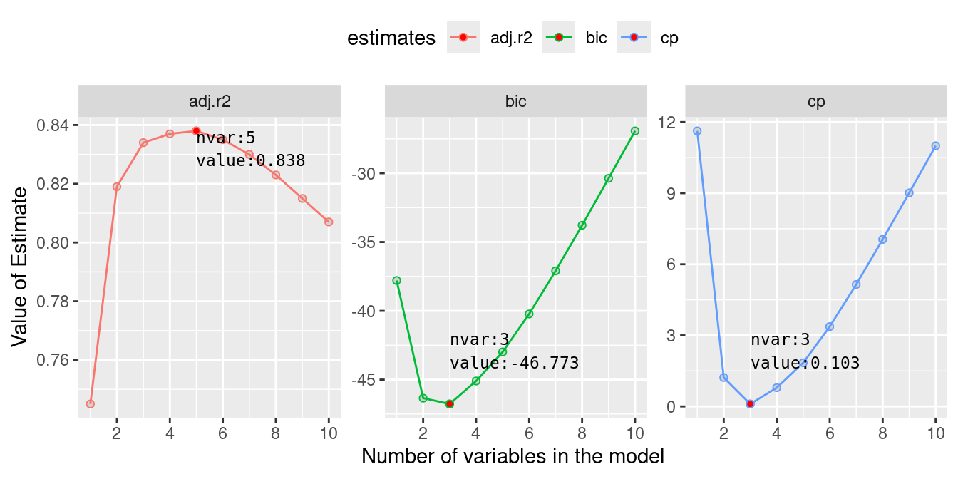
We can make a plot to visualise the properties of these individual models and select a model with specific number of predictor that can give minimum BIC, or minimum CP or maximum adjusted rsquared.

library(ggplot2)
library(dplyr)
bs.est.select <- bs.est %>%
  group_by(estimates) %>%
  filter(
    (value == max(value) & estimates == "adj.r2") |
    (value == min(value) & estimates != "adj.r2")
  )
assessment.plt <- ggplot(bs.est, aes(nvar, value, color = estimates)) +
  geom_point(shape = 21, fill = "lightgray") +
  geom_line() +
  facet_wrap(~estimates, scale = 'free_y') +
  theme(legend.position = "top") +
  labs(x = "Number of variables in the model",
       y = "Value of Estimate") +
  scale_x_continuous(breaks = seq(0, 10, 2)) +
  geom_point(data = bs.est.select, fill = "red",
             shape = 21) +
  geom_text(aes(label = paste0("nvar:", nvar, '\n', "value:", value)),
            data = bs.est.select, 
            size = 3, hjust = 0, vjust = c(1, -1, -1),
            color = "black", family = "monospace")

From these plots, we see that with 5 variables we will obtain maximum adjusted coefficient of determination (\(R^2\)). Similarly, both BIC and Mallow CP will be minimum for models with only 3 predictor variables. With the help of table above, we can identify these variables. From the table, row corresponding to 3 variables, we see that the three predictors are wt, qsec and am. To obtain maximum adjusted \(R^2\), disp and hp should be added to the previous 3 predictors.

This way, we can reduce a model to few variables optimising different assessment criteria. Let look at the fit of these reduced models:

model.3 <- lm(mpg ~ wt + qsec + am, data = mtcars)
model.5 <- update(model.3, . ~ . + disp + hp)

Summaries of the models

3 Variable Model

summary(model.3)


Call:
lm(formula = mpg ~ wt + qsec + am, data = mtcars)

Residuals:
    Min      1Q  Median      3Q     Max 
-3.4811 -1.5555 -0.7257  1.4110  4.6610 

Coefficients:
            Estimate Std. Error t value Pr(>|t|)    
(Intercept)   9.6178     6.9596   1.382 0.177915    
wt           -3.9165     0.7112  -5.507 6.95e-06 ***
qsec          1.2259     0.2887   4.247 0.000216 ***
am            2.9358     1.4109   2.081 0.046716 *  
---
Signif. codes:  0 '***' 0.001 '**' 0.01 '*' 0.05 '.' 0.1 ' ' 1

Residual standard error: 2.459 on 28 degrees of freedom
Multiple R-squared:  0.8497,    Adjusted R-squared:  0.8336 
F-statistic: 52.75 on 3 and 28 DF,  p-value: 1.21e-11

5 Variable Model

summary(model.5)


Call:
lm(formula = mpg ~ wt + qsec + am + disp + hp, data = mtcars)

Residuals:
    Min      1Q  Median      3Q     Max 
-3.5399 -1.7398 -0.3196  1.1676  4.5534 

Coefficients:
            Estimate Std. Error t value Pr(>|t|)   
(Intercept) 14.36190    9.74079   1.474  0.15238   
wt          -4.08433    1.19410  -3.420  0.00208 **
qsec         1.00690    0.47543   2.118  0.04391 * 
am           3.47045    1.48578   2.336  0.02749 * 
disp         0.01124    0.01060   1.060  0.29897   
hp          -0.02117    0.01450  -1.460  0.15639   
---
Signif. codes:  0 '***' 0.001 '**' 0.01 '*' 0.05 '.' 0.1 ' ' 1

Residual standard error: 2.429 on 26 degrees of freedom
Multiple R-squared:  0.8637,    Adjusted R-squared:  0.8375 
F-statistic: 32.96 on 5 and 26 DF,  p-value: 1.844e-10

From these output, it seems that although adjusted \(R^2\) has increased in later model, the additional variables are not significant. we can compare these two model with an ANOVA test which compares the residual variance between these two models. We can write the hypothesis as,

\(H_0:\) Model 1 and Model 2 are same vs \(H_1:\) Model 1 and Model 2 are different

where, Model 1 and Model 2 represents 3 variable and 5 variable model

anova(model.3, model.5)

Analysis of Variance Table

Model 1: mpg ~ wt + qsec + am
Model 2: mpg ~ wt + qsec + am + disp + hp
  Res.Df    RSS Df Sum of Sq      F Pr(>F)
1     28 169.29                           
2     26 153.44  2    15.848 1.3427 0.2786

The ANOVA result can not reject the hypothesis so claim that Model 1 and Model 2 are same. So, it is better to select the simpler model with 3 predictor variables.

Step-wise selection

When the number of increases, a exhaustive search of all possible subset is computationally intensive. This disadvantage can be overcome by using step-wise selection procedure. A step-wise variable selection procedure can be,

Forward Selection Procedure: In this procedure …
Backward Elimination Procedure: Here …