A biplot is a powerful graphical tool that represents data in two dimensions, where both the observations and variables are represented. Biplots are particularly useful for multivariate data, allowing users to examine relationships between variables and identify patterns.
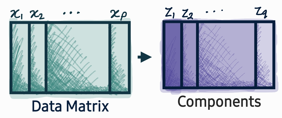
Consider a data matrix \(\mathbf{X}_{n\times p}\) with \(p\) variables and \(n\) observations. To explore the data further with biplot, principal component analysis (PCA) is used here.
Principal component analysis (PCA) compresses the variance of the data matrix to create a new set of orthogonal (linearly independent) variables \(\mathbf{Z} = \begin{pmatrix}\mathbf{z}_1 & \mathbf{z}_2 & \ldots & \mathbf{z}_q\end{pmatrix}\), where \(q = \min(n, p)\), often termed as principal components (PC) or scores. In PCA, the most variation is captured by the first component and rest in the subsequent components in decreasing order. In other words, the first principal component (\(\mathbf{z}_1\)) captures the highest variation and second principal component (\(\mathbf{z}_2\)) captures the maximum of remaing variation and so on.
We can use eigenvalue decomposition or singular value decompostion for this purpose.
These principle components are created using linear combination of the original variables. For example, \(\mathbf{z}_1 = w_{11}\mathbf{x}_1 + \ldots + w_{1p}\mathbf{x}_p\) and similarly for \(\mathbf{z}_2, \ldots, \mathbf{z}_q\). Here we can estimate weights \(w_{ij}\), where \(i = 1 \ldots q\) and \(j = 1 \ldots p\) using eigenvalue decomposition or singular value (SVD). These weights are also refered as loading or the matrix of these weights as rotation matrix.
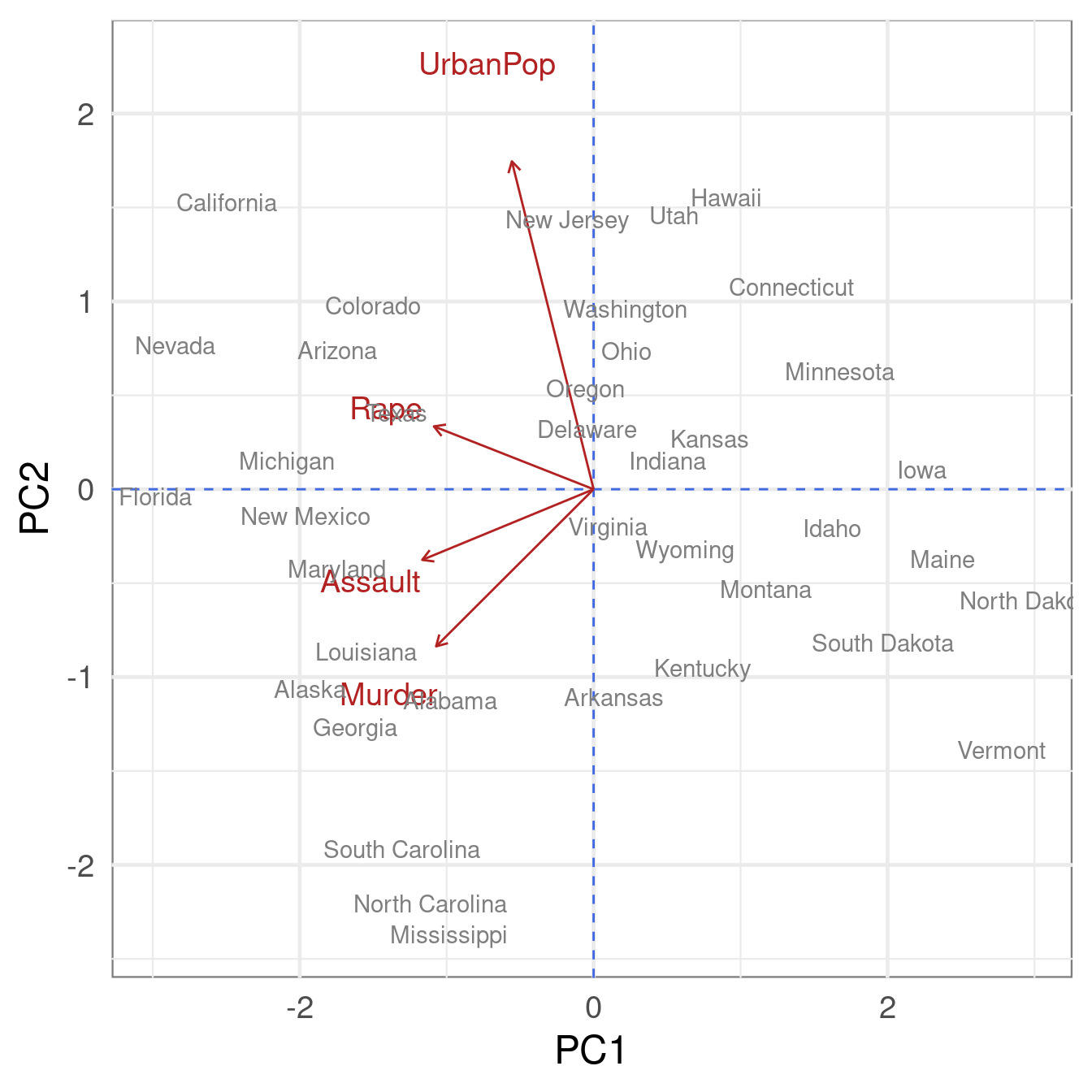
Biplot plots the scores from two principal components together with loadings (weight) for each variables in the same plot. The following example uses USArrests data from datasets package in R. The dataset contains the number of arrests per 100,000 residents for assault, murder, and rape in each of the 50 US states in 1973.
Two functions prcomp and princomp in R performs the principal component analysis. The function prcomp uses SVD on data matrix \(\mathbf{X}\) while princomp uses eigenvalue decomposition on covariance or correlation matrix of the data matrix. We will use prcomp for our example.
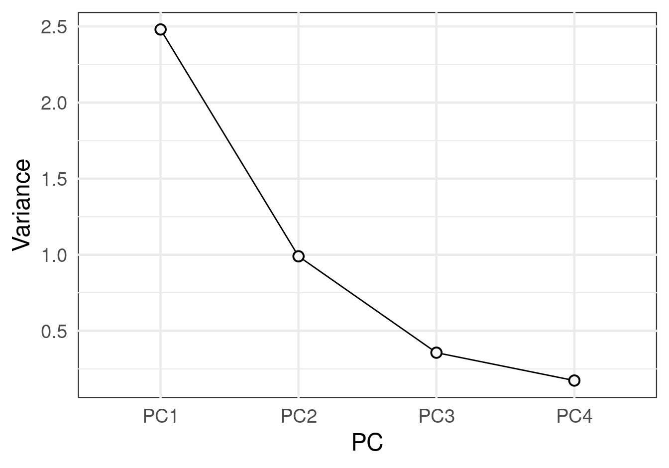
Here we see that more than 87% of variation in \(\mathbf{X}\) was captured by first two principal components (65% by the first and 25% by the second component).
Explore data using biplot
Now lets compare the scores from the first two components, observations and variables in the data matrix. From the USArrests data, lets look at the top five states with highest and lowest arrest for each of these crimes.
# A tidytable: 5 × 5
  State          Murder Assault UrbanPop  Rape
  <chr>           <dbl>   <int>    <int> <dbl>
1 Vermont           2.2      48       32  11.2
2 West Virginia     5.7      81       39   9.3
3 Mississippi      16.1     259       44  17.1
4 North Dakota      0.8      45       44   7.3
5 North Carolina   13       337       45  16.1
Code
USArrests %>%arrange(Rape) %>%top_n()
# A tidytable: 5 × 5
  State         Murder Assault UrbanPop  Rape
  <chr>          <dbl>   <int>    <int> <dbl>
1 North Dakota     0.8      45       44   7.3
2 Maine            2.1      83       51   7.8
3 Rhode Island     3.4     174       87   8.3
4 West Virginia    5.7      81       39   9.3
5 New Hampshire    2.1      57       56   9.5
Comparing these highest and lowest arrests with the biplot, we can see a pattern. The weights corresponding to PC1 for all the variables are negative and are directed towards states like Florida, Nevada, and California. These states have the highest number of arrests for all of these crimes where as states that are in the oppositve direction like Iowa, North Dakota, and Vermont have the lowest arrest.
Similarly, UrbanPop have the highest weights corresponding to PC2 so the states in that direction such as California, Hawaii, and New Jersey have highest arrest related to UrbanPop. The states in the opposite direction, i.e. with negative PC2 scores such as Mississippi, North Carolina, Vermont, and South Carolina have the lowest arrest related to UrbanPop.
The weights for all variables are negative and towards states like . So in our data these states must have the highest arrests in all these crimes where as states like New Dakota, Vermont, and Iowa have the lowest arrests.